아래의 모든 내용은 파이썬으로 데이터 주무르기(저자 민형기)의 예시를 사용했습니다.
▶ 몇 개의 사인 함수 그리기
import matplotlib.pyplot as plt
%matplotlib inline

import seaborn as sns

x = np.linspace(0, 14, 100)
y1 = np.sin(x)
y2 = 2*np.sin(x+0.5)
y3 = 3*np.sin(x+1.0)
y4 = 4*np.sin(x+1.5)

plt.figure(figsize=(10,6))
plt.plot(x,y1, x,y2, x,y3, x,y4)
plt.show()
▶ Seaborn의 white 스타일 지원
sns.set_style("white")

plt.figure(figsize=(10,6))
plt.plot(x,y1, x,y2, x,y3, x,y4)

sns.despine()

plt.show()
▶ Seaborn의 dark 스타일 지원
sns.set_style("dark")

plt.figure(figsize=(10,6))
plt.plot(x,y1, x,y2, x,y3, x,y4)
plt.show()
▶ Seaborn의 whitegrid 스타일 지원
sns.set_style("whitegrid")

plt.figure(figsize=(10,6))
plt.plot(x,y1, x,y2, x,y3, x,y4)
plt.show()
▶ Seaborn의 despine옵션, 축을 살짝 벌린다
plt.figure(figsize=(10,6))
plt.plot(x,y1, x,y2, x,y3, x,y4)

sns.despine(offset=10)

plt.show()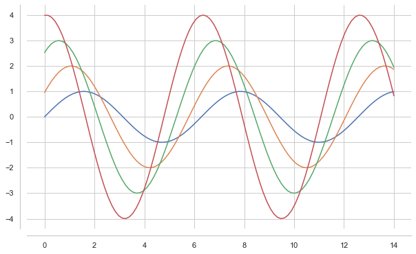
▶ Seaborn 내 연습할 만한 데이터, Tips 데이터 셋 불러오기
import matplotlib.pyplot as plt
import numpy as np
import seaborn as sns

sns.set_style("whitegrid")
%matplotlib inline
tips = sns.load_dataset("tips")
tips.head(5)
▶ Seaborn boxplot 그리기
sns.set_style("whitegrid")

plt.figure(figsize=(8,6))
sns.boxplot(x=tips["total_bill"])
plt.show()
▶ Seaborn boxplot 그리기 2
plt.figure(figsize=(8,6))
sns.boxplot(x="day", y="total_bill", data=tips)
plt.show()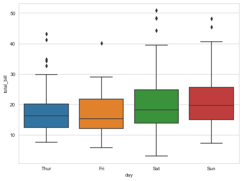
▶ Seaborn hue 옵션 이용해 구분하기, 흡연 여부 구별
plt.figure(figsize=(8,6))
sns.boxplot(x="day", y="total_bill", hue="smoker", data=tips, palette="Set3") # palette는 색상
plt.show()
▶ Seaborn swarmplot 그리기
plt.figure(figsize=(8,6))
sns.swarmplot(x="day", y="total_bill", data=tips, color=".5")
plt.show()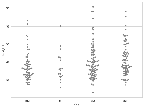
▶ Seaborn swarmplot, boxplot 동시에 그리기
plt.figure(figsize=(8,6))
sns.boxplot(x="day", y="total_bill", data=tips)
sns.swarmplot(x="day", y="total_bill", data=tips, color=".25")
plt.show()
▶ Seaborn lmplot 그리기
# 데이터를 scatter처럼 그리고 직선으로 regression한 그림도 같이 그려주고 유효범위 ci로 잡아줌
sns.set_style("darkgrid")
sns.lmplot(x="total_bill", y="tip", data=tips, size=7)
plt.show()
▶ Seaborn lmplot hue 옵션 추가하기
sns.lmplot(x="total_bill", y="tip", hue="smoker", data=tips, size=7)
plt.show()
▶ Seaborn lmplot palette로 색상지 정하기
sns.lmplot(x="total_bill", y="tip", hue="smoker", data=tips, palette="Set1", size=7)
plt.show()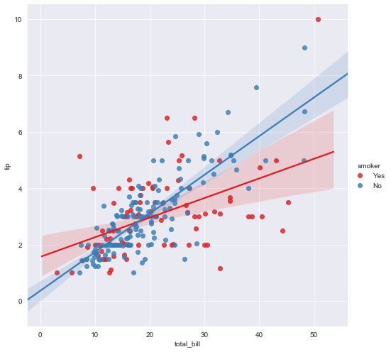
▶ Numpy 데이터 생성
uniform_data = np.random.rand(10, 12)
uniform_data
▶ Seaborn heatmap 도구 사용
sns.heatmap(uniform_data)
plt.show()
▶ Seaborn heatmap bar 편집
sns.heatmap(uniform_data, vmin=0, vmax=1)
plt.show()
▶ Seaborn flights 데이터 불러오기
flights = sns.load_dataset("flights")
flights.head(5)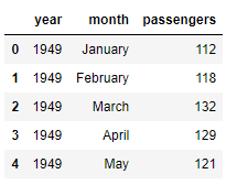
▶ Pivot 기능으로 월별, 연도별 구별하기
flights = flights.pivot("month", "year", "passengers")
flights.head(5)
▶ Seaborn heatmap으로 적용하기
plt.figure(figsize=(10,8))
sns.heatmap(flights)
plt.show()
▶ Seaborn heatmap annot, fmt 추가 옵션 적용하기
plt.figure(figsize=(10,8))
sns.heatmap(flights, annot=True, fmt="d")
plt.show()
▶ Seaborn style ticks로 iris데이터 불러오기
sns.set(style="ticks")
iris = sns.load_dataset("iris")
iris.head(10)
▶ Seaborn pairplot 그리기
sns.pairplot(iris)
plt.show()
▶ Seaborn pairplot hue 옵션 추가
sns.pairplot(iris, hue="species")
plt.show()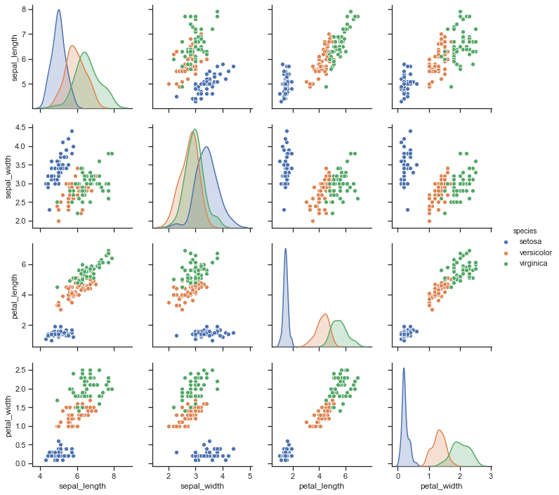
▶ Seaborn pairplot 몇 가지 변수만 적용하기
sns.pairplot(iris, vars=["sepal_width", "sepal_length"])
plt.show()
▶ Seaborn pairplot 변수 구체적으로 적용하기
sns.pairplot(iris, x_vars=["sepal_width", "sepal_length"],
             y_vars=["petal_width", "petal_length"])
plt.show()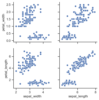
▶ Seaborn anscombe 데이터 불러오기
anscombe = sns.load_dataset("anscombe")
anscombe.head(5)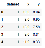
▶ Seaborn lmplot 적용하기
sns.set_style("darkgrid")

sns.lmplot(x="x", y="y", data=anscombe.query("dataset == 'I'"),  ci=None, size=7)
plt.show()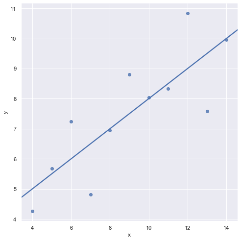
▶ Seaborn lmplot scatter_kws 옵션으로 포인트 키우기
sns.lmplot(x="x", y="y", data=anscombe.query("dataset == 'I'"),
           ci=None, scatter_kws={"s": 80}, size=7)
plt.show()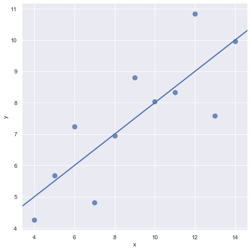
▶ Seaborn lmplot 데이터셋 변경 적용하기
sns.lmplot(x="x", y="y", data=anscombe.query("dataset == 'II'"),
           order=1, ci=None, scatter_kws={"s": 80}, size=7)
plt.show()
▶ Seaborn lmplot order 옵션 변경 적용하기
sns.lmplot(x="x", y="y", data=anscombe.query("dataset == 'II'"),
           order=2, ci=None, scatter_kws={"s": 80}, size=7)
plt.show()
▶ Seaborn lmplot 데이터 변경 3
sns.lmplot(x="x", y="y", data=anscombe.query("dataset == 'III'"),
           ci=None, scatter_kws={"s": 80}, size=7)
plt.show()
▶ Seaborn lmplot robust 옵션 추가
sns.lmplot(x="x", y="y", data=anscombe.query("dataset == 'III'"),
           robust=True, ci=None, scatter_kws={"s": 80}, size=7)
plt.show()
여기까지가 Seaborn에 대한 간략한 예시였습니다. 감사합니다.
'Python > 라이브러리' 카테고리의 다른 글
| Pandas 고급 (0) | 2019.09.25 |
|---|---|
| 파이썬의 대표 시각화 도구 Matplotlib (0) | 2019.09.17 |
| Pandas 기초 익히기 (0) | 2019.09.16 |


댓글